Double Pendulum · Ian Wood

The system and its boundary

The application solves two ideal conservative systems: a simple double pendulum with endpoint masses, and a compound model with extended rigid bodies and explicit centres of mass. Damping, forcing, friction, and measurement error are outside both formulations.

The angles \(q=(\theta_1,\theta_2)\) are the generalised coordinates. A complete state also contains angular velocities or canonical momenta. From selected parameters and initial conditions, the application computes one trajectory for animation, angle traces, and state-space projections.

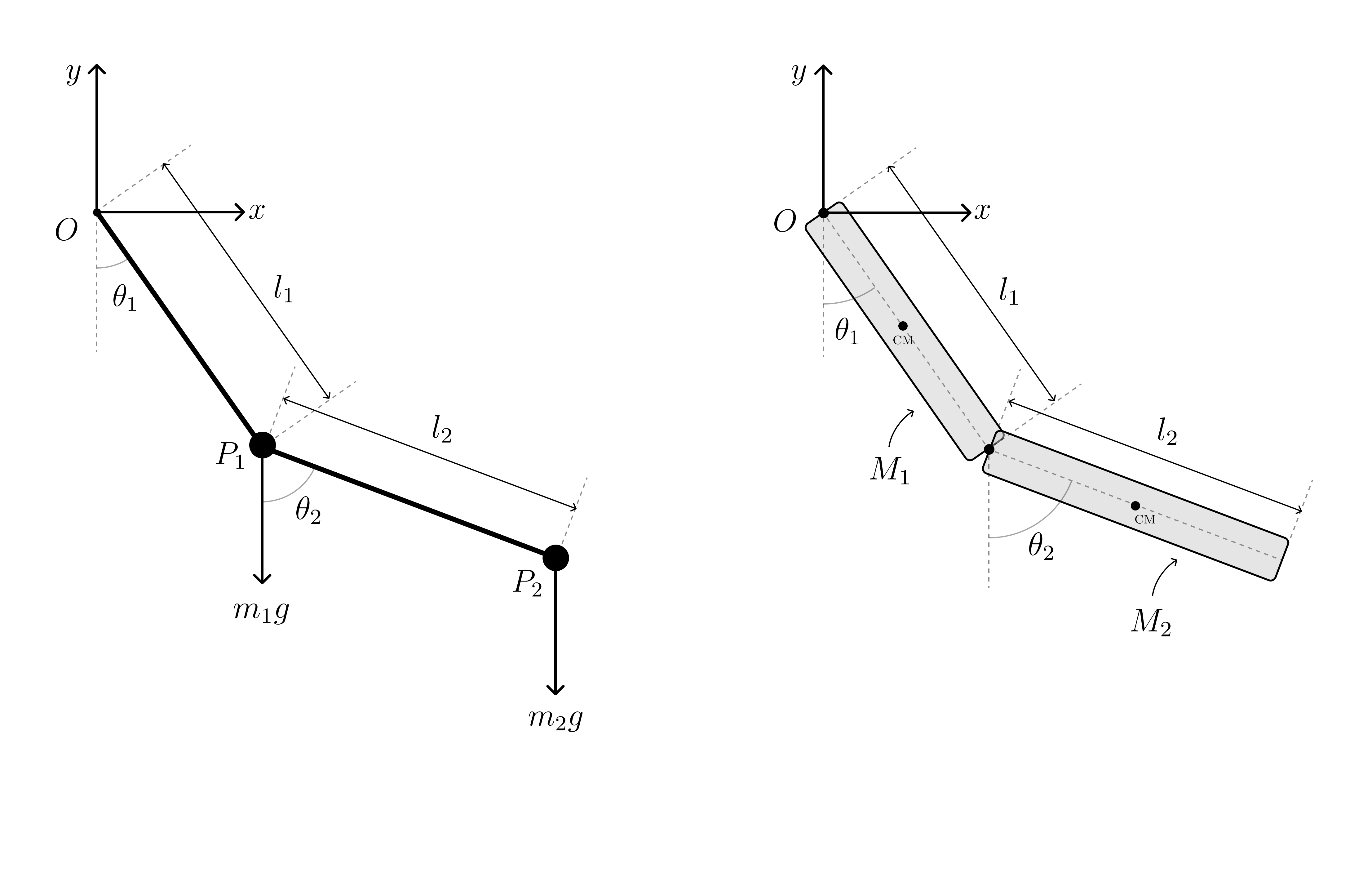
Side-by-side schematic of the implemented simple and compound double pendulums, with their lengths, angles, masses, centres of mass, forces, and moments labelled. — The simple model uses point masses; the compound model uses extended links with centres of mass and moments. This schematic explains the geometry rather than a numerical result.

Two formulations of the same motion

Lagrangian formulation

The Lagrangian route begins with kinetic and potential energy. The Euler–Lagrange equations give the coupled equations of motion:

\[ L(q,\dot q)=T(q,\dot q)-V(q), \qquad \frac{d}{dt}\left(\frac{\partial L}{\partial \dot q_i}\right) -\frac{\partial L}{\partial q_i}=0. \]

Hamiltonian formulation

The Hamiltonian route introduces canonical momenta \(p_i=\partial L/\partial \dot q_i\) and evolves four first-order equations:

\[ H(q,p)=\sum_i p_i\dot q_i-L(q,\dot q), \qquad \dot q_i=\frac{\partial H}{\partial p_i}, \qquad \dot p_i=-\frac{\partial H}{\partial q_i}. \]

The interface keeps the selected formulation visible because the two routes describe the same mechanics with different state variables.

Computational approach

SymPy derives and caches the governing expressions for the selected model. Each formulation is arranged as a first-order state derivative and passed to SciPy’s solve_ivp. The Lagrangian state contains angles and angular velocities; the Hamiltonian state contains angles and canonical momenta.

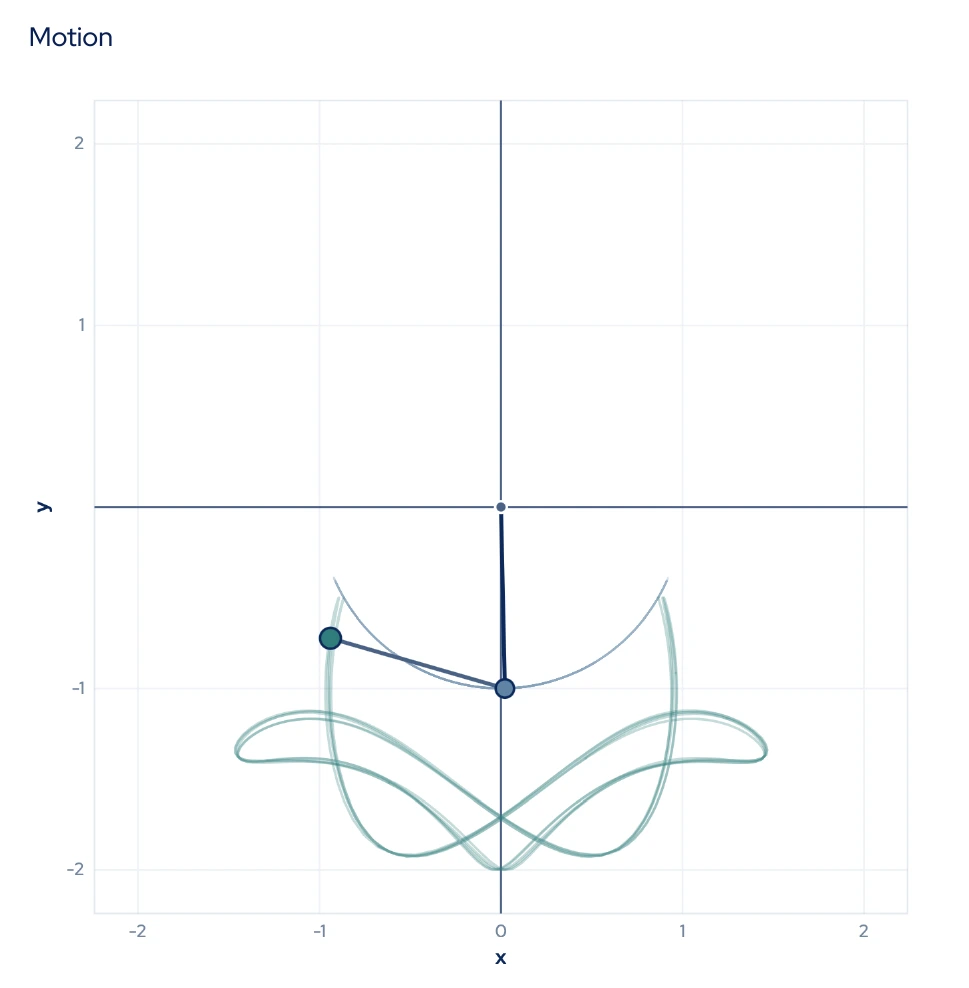
The requested evaluation times provide a common basis for Cartesian animation, angle traces, and angular or phase projections. Visitors can change the model, formulation, physical parameters, initial conditions, and integration time; every view then updates from the same solution.

Computed Cartesian motion for a 20-second simple Hamiltonian run with initial angles of zero and 120 degrees. — Simple Hamiltonian model; gravity 9.81 m/s²; unit lengths and masses; initial angles 0° and 120°; zero initial angular velocities. This is one trajectory, not a solver-validation or chaos test.

Limitations

The application is for mathematical exploration, not a calibrated physical apparatus. Numerical validation remains incomplete: it does not yet publish a finished suite for solver convergence, conservation error, agreement between formulations, or defined chaos diagnostics. A complicated trajectory alone is not treated as evidence of chaos.