Numerical optimisation
Nonlinear Optimisation
Custom Newton–Raphson and Levenberg–Marquardt solvers tested on Himmelblau's function and other nonlinear objectives.
Educational study
Finding a local minimiser
This project is an educational implementation of methods for unconstrained nonlinear optimisation. It asks how Newton–Raphson and a damped Levenberg–Marquardt method behave when their gradients, Hessians, and linear solves are made explicit rather than hidden behind a library call.
The Python code accepts a SymPy expression, differentiates it symbolically, and evaluates the resulting objective, gradient, and Hessian numerically. A custom \(LDL^{\mathsf T}\) decomposition and triangular substitutions solve the linear systems used at each step. The notebook compares both custom solvers with SciPy’s BFGS implementation on several named test functions.
Two second-order approaches
Newton–Raphson solves the local quadratic model
If the decomposed Hessian is not positive definite, the implementation shifts it by a multiple of the identity before solving. The Levenberg–Marquardt solver uses a damped Hessian instead. It compares the actual reduction in the objective with the reduction predicted by the quadratic model, rejects weak steps, and adjusts the damping parameter for the next iteration. Both solvers stop only when gradient norm, step size, and change in objective pass their tolerances.
Himmelblau’s function
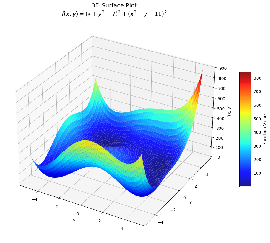
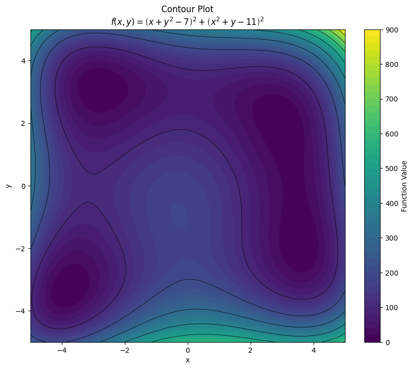
Himmelblau’s function is the clearest two-dimensional test in the notebook:
Its four local minima lie near \((3,2)\), \((-2.805,3.131)\), \((-3.779,-3.283)\), and \((3.584,-1.848)\). The surface shows why a local method must be interpreted together with its starting point; the contour view makes the four basins easier to distinguish.
Starting at \((0,0)\), all three methods recorded convergence to \((3,2)\):
Objective surface
Objective contours
| Method | Recorded minimiser | \(f(x,y)\) | Iterations |
|---|---|---|---|
| Levenberg–Marquardt | \((3.00000002, 1.99999994)\) | \(4.87\times10^{-14}\) | 9 |
| Newton–Raphson | \((3,2)\) | \(0\) | 12 |
| SciPy BFGS | \((2.99999994, 1.99999999)\) | \(1.38\times10^{-13}\) | 10 |
These are the saved notebook results for one starting point, not a general ranking of the algorithms. The notebook also starts Levenberg–Marquardt near each visible basin and recovers all four minima.
Limitations
This is a small-scale learning project, not a general optimisation package. It covers unconstrained local minimisation and uses symbolic derivatives, so it is not designed for large, sparse, or non-symbolic problems. Convergence depends on the initial point and local curvature. The notebook's iteration and function-evaluation counts come from different implementations and are not a timing benchmark. Constraints, global-search guarantees, and a systematic performance study are not implemented.