Population Dynamics

Four implemented model families

Population Dynamics Explorer implements four families: continuous differential equations, discrete maps, interacting populations, and probabilistic branching processes. Each route pairs model-specific controls with the relevant equilibria, stability calculations, trajectories, phase portraits, or ensemble summaries.

Continuous models

The spruce budworm outbreak model is the principal continuous example. After scaling population to \(u\) and time to \(\tau\), logistic growth competes with a saturating predation response:

\[ \frac{\mathrm du}{\mathrm d\tau} =ru\left(1-\frac{u}{q}\right)-\frac{u^2}{1+u^2}. \]

Here \(r\) is the dimensionless growth parameter and \(q\) the capacity ratio. The model can have one or three positive equilibria; with three, the unstable middle state separates low-density and outbreak basins. The application finds and classifies these equilibria and computes a fixed-\(q\) bifurcation sweep.

At \(q=13\), stable and unstable branches meet at two folds. The selected \(r=0.44\) therefore lies in a bistable interval with three positive equilibria.

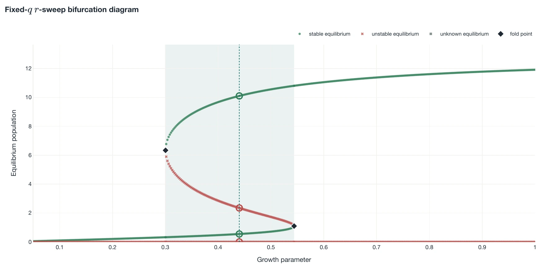
Fixed-q bifurcation diagram for the spruce budworm model, showing stable and unstable branches, two folds, and the selected growth parameter. — Spruce budworm outbreak model
At q = 13, the marker r = 0.44 lies between the two folds, where three equilibria coexist. This is nondimensional model output, not population data.

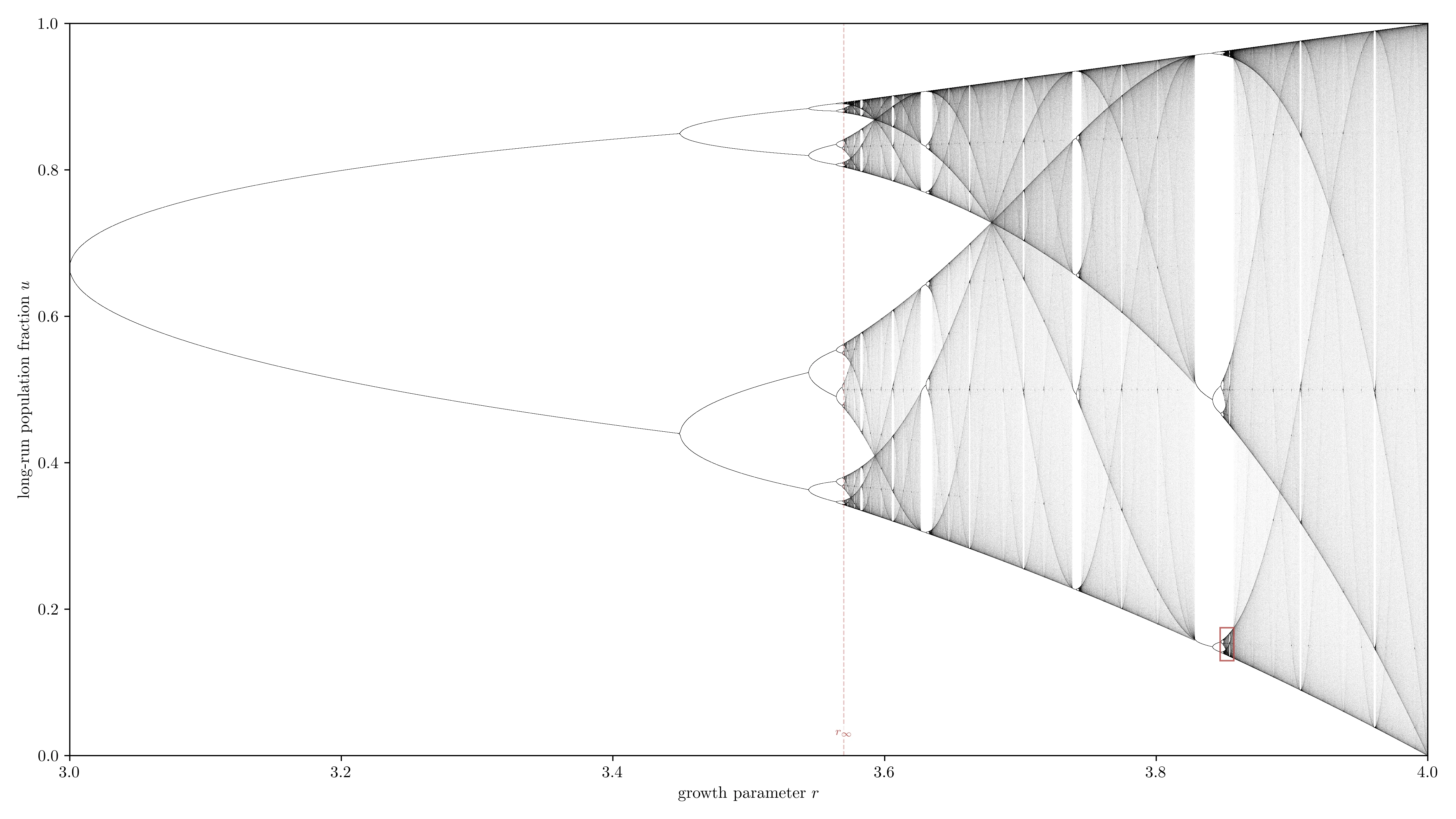
Logistic-map bifurcation diagram from r equals 3 to 4, showing period doubling, chaotic bands, and periodic windows. — Logistic-map bifurcation
Sampled long-run states show period doubling, chaotic bands, and periodic windows across 3 ≤ r ≤ 4.

Discrete models

For populations updated in separate steps, the normalised logistic map is

\[ u_{n+1}=F(u_n)=r u_n(1-u_n), \qquad 0\leq u_n\leq 1. \]

The orbit records successive states, while the cobweb shows the same updates between \(y=F(u)\) and \(y=u\). Fixed points are locally attracting when \(\lvert F’(u^{\ast})\rvert<1\); higher iterates and cycle multipliers test periodic states. The full sweep shows the loss of fixed-point stability and the periodic windows inside chaotic bands.

Interacting populations

The saturating predator-prey model is the principal interacting example. Its nondimensional equations are

\[ \frac{\mathrm du}{\mathrm d\tau}=u(1-u)-\frac{auv}{u+d}, \qquad \frac{\mathrm dv}{\mathrm d\tau}=bv\left(1-\frac{v}{u}\right). \]

The parameters set predation intensity, predator response, and saturation. The application finds the positive coexistence point and computes the Hopf threshold \(b_{\mathrm{Hopf}}\) for the selected \((a,d)\), connecting the controls to stable or unstable coexistence.

The figure uses \(a=1\), \(d=0.1\), and \(b=1.5b_{\mathrm{Hopf}}\). Trajectories spiral towards the coexistence point \((0.27016,0.27016)\) with decaying oscillations. The solver excludes the singular boundary \(u=0\) from the biological domain.

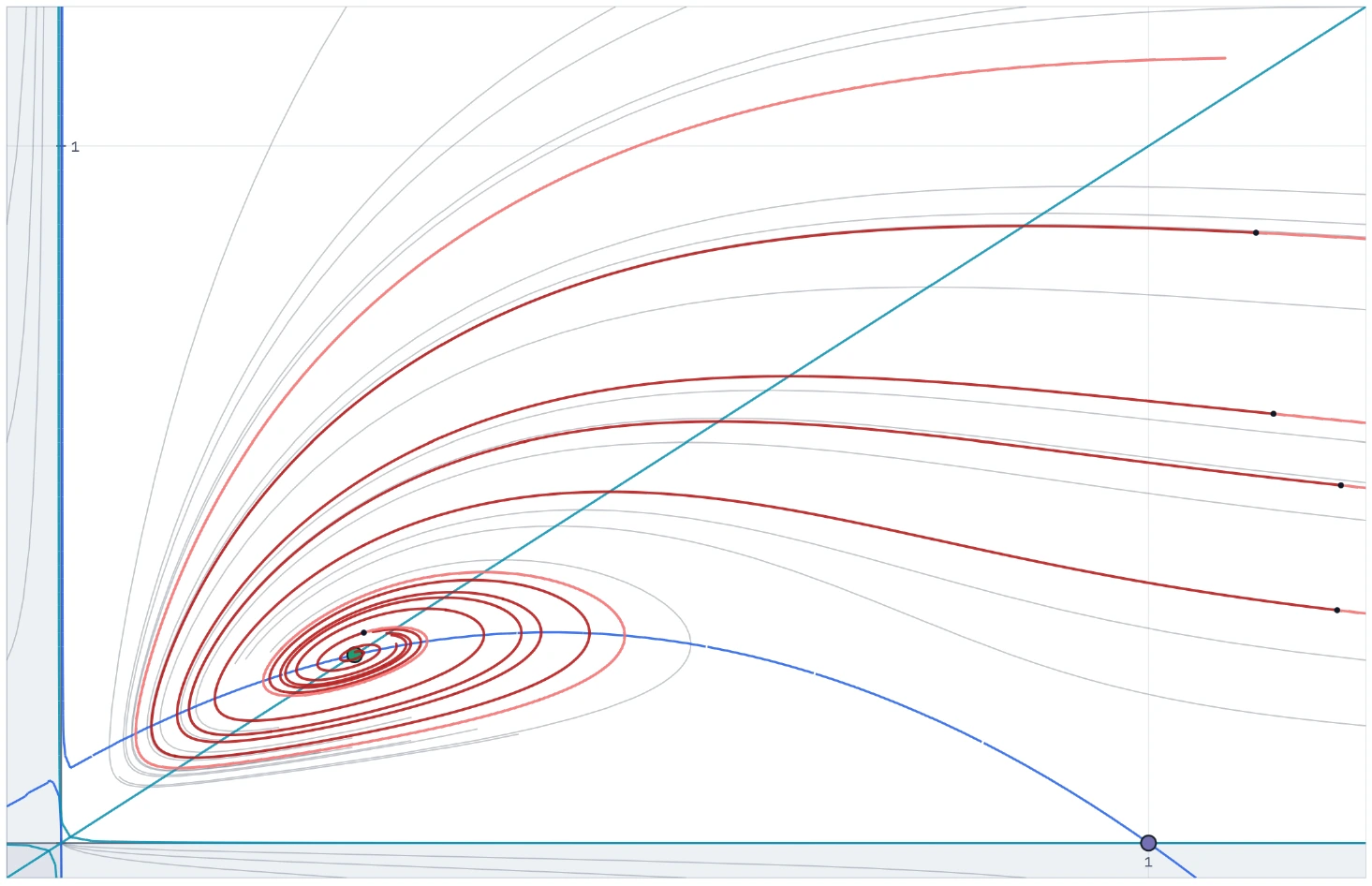
Saturating predator-prey phase portrait with nullclines, a coexistence equilibrium, and trajectories spiralling towards it. — Saturating predator-prey model
The nullclines locate coexistence; the selected trajectories show damped oscillations converging to it.

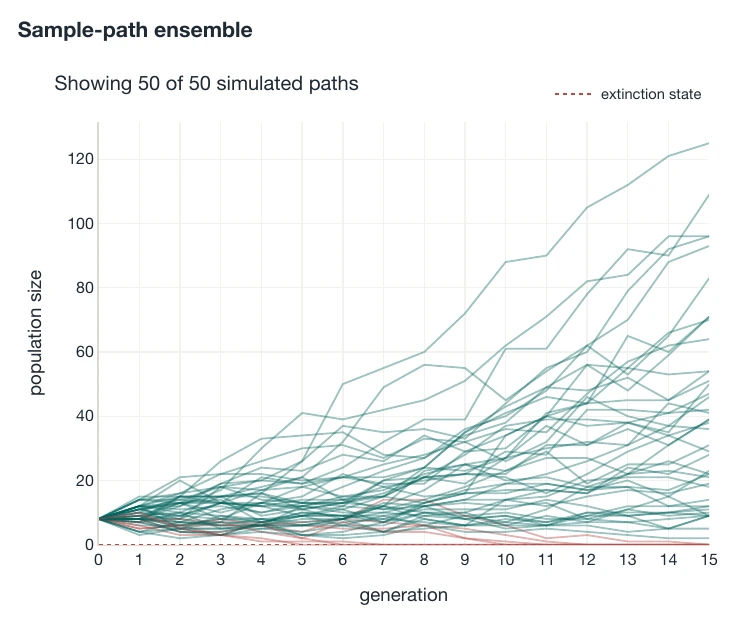
Galton-Watson sample-path ensemble showing 50 simulated population trajectories over 15 generations, with seven reaching the extinction state. — Poisson branching-process ensemble
From Z₀ = 8 and mean offspring 1.1, 50 seeded realisations are followed for 15 generations; 7 are extinct by the horizon.

Probabilistic models

The Galton-Watson branching process follows a population generation by generation. Each of the \(Z_{n-1}\) individuals independently produces an offspring count \(Y_{n,i}\):

\[ Z_n=\sum_{i=1}^{Z_{n-1}}Y_{n,i}, \qquad Z_n=0\Longrightarrow Z_{n+1}=0. \]

Choosing an offspring law, its mean, the initial population, a generation horizon, an ensemble size, and a random seed defines one experiment. The explorer plots the offspring distribution and sample-path ensemble, then reports extinction, censoring, and horizon-survivor counts. In the selected Poisson experiment, 7 of 50 paths are extinct by generation 15. A path still alive at the horizon is not claimed to survive forever.

What the visitor can change

Each route exposes only its relevant parameters and initial conditions. The spruce budworm view controls growth, capacity, and the bifurcation sweep; the logistic view controls the update parameter, iterations, cycle length, and range; the predator-prey view controls \(a\), \(d\), and \(b/b_{\mathrm{Hopf}}\), with phase-plane clicks adding initial populations. The branching-process view controls the offspring law and mean, initial population, horizon, ensemble size, and seed.

Limitations

The explorer supports qualitative mathematics and finite numerical experiments, not empirical validation or complete coverage of population processes. Probabilistic results describe the selected ensemble and horizon: a path alive at the final displayed generation is not shown to survive forever, while censored paths are excluded from extinction and exact horizon counts.